43 change pivot table labels
How to reset a custom pivot table row label Drag the row field out of the pivot table. Right click on the pivot table and select ' Refresh '. Drag the row field back onto the pivot table. stackoverflow.com/questions/998185/excel-pivot-table-row-labels-not-refreshing Proposed as answer by Tarvaa Friday, February 12, 2016 1:07 PM Tuesday, December 17, 2013 10:19 AM 0 Sign in to vote support.google.com › looker-studio › answerPivot table reference - Looker Studio Help - Google Pivot tables in Looker Studio. Pivot tables in Looker Studio take the rows in a standard table and pivot them so they become columns. This lets you group and summarize the data in ways a standard table can't provide. Example: The following is a standard table listing the Revenue Per User metric by calendar quarter and year:
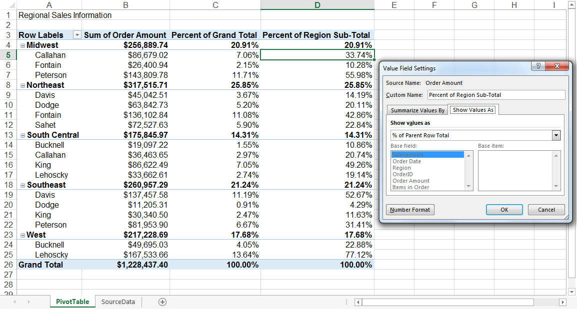
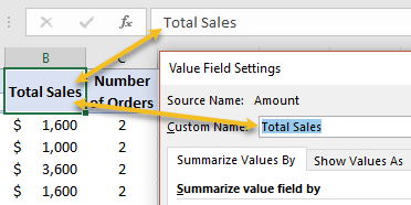
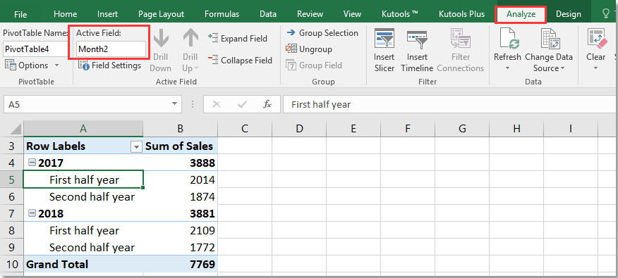
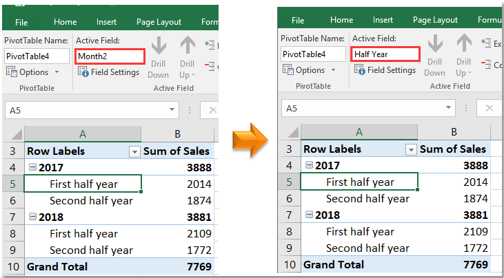
Rename a field or item in a PivotTable or PivotChart Go to PivotTable Tools > Analyze, and in the Active Field group, click the Active Field text box. If you're using Excel 2007-2010, go to PivotTable Tools > Options. Type a new name. Press ENTER. Note: Renaming a numeric item changes it to text, which sorts separately from numeric values and can't be grouped with numeric items. PivotChart report

Change pivot table labels
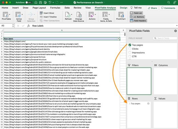
Pivot Table shows row labels instead of field name - YouTube 00:00 Pivot table not showing column names, says 'Row Labels'00:13 Remove 'Row Labels', leave blank00:20 Show the column names in the Pivot TableChange your ... Change row label in Pivot Table with VBA | MrExcel Message Board If they appear as columns they are not row labels. If you want to change a field name between the source table and the pivot table I suggest you do this in SQL. So if the source data has fields Type and Manufacturer but you want them to be Type and Country in the pivot table it'd be like this, SELECT Type, Manufacturer AS [Country] › excel-pivot-table-subtotalsExcel Pivot Table Subtotals Examples Videos Workbooks Oct 10, 2022 · In the pivot table below, the Technician Count field was added below District, and the District field now has a subtotal after each District name. Hide All Subtotals. In a new pivot table, when you add multiple fields to the Row Labels or column Labels areas, subtotals are automatically shown for the outer fields.
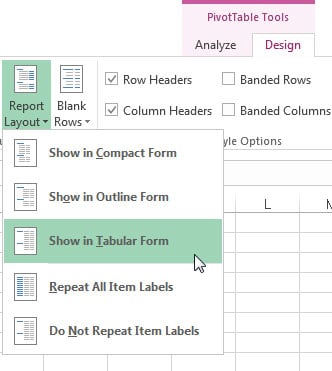
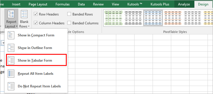
Change pivot table labels. Pivot Table Row Labels - Microsoft Community If you go to PivotTable Tools > Analyze > Layout > Report Layout > Show in Tabular Form, your column headers will be used for the row labels. Every once in a while there's a sudden gust of gravity... Report abuse 1 person found this reply helpful · Was this reply helpful? Yes No A. User Replied on December 19, 2017 Change the pivot table "Row Labels" text | MrExcel Message Board 144. Feb 4, 2021. #3. mart37 said: Click on the cell and typ the text. Thanks mart37. So simple! I was looking for a way to change it on the ribbons & settings. Typical Excel - things you think are difficult are easy, and things that should be easy are difficult! Quick tip: Rename headers in pivot table so they are presentable Just type over the headers / total fields to make them user friendly. See this quick demo to understand what I mean: So simple and effective. Keep in mind: You can not rename to an existing column data in your data. So if you want to rename to "Amount" which is a field in the data table, simply type "Amount " with an extra space at end. How to Customize Your Excel Pivot Chart Data Labels - dummies For example, if you want to label data markers with a pivot table chart using data series names, select the Series Name check box. If you want to label data markers with a category name, select the Category Name check box. To label the data markers with the underlying value, select the Value check box.
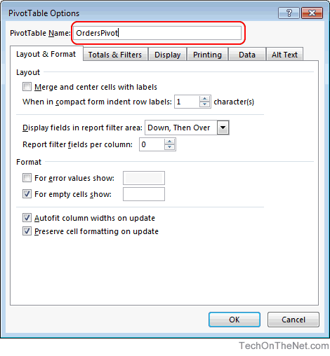
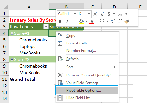
Change Blank Labels in a Pivot Table - Contextures Blog You can manually change the (blank) labels in the Row or Column Labels areas by typing over them in the pivot table. You can type any text to replace the (Blank) entry, even a space character, but you can't clear the cell and leave it empty: Select one of the Row or Column Labels that contains the text (blank). techcommunity.microsoft.com › t5 › excelPasting Pivot Table as Values... losing Borders and formatting Feb 16, 2018 · You can share a Pivot Table with the formatting without the underlying data. In the Pivot Table Options, Data Tab, de-select the option "Save source data with the file", you can do this before or after sending the worksheet to a new Workbook that you will use for distribution. Pivot table row labels in separate columns • AuditExcel.co.za Our preference is rather that the pivot tables are shown in tabular form (all columns separated and next to each other). You can do this by changing the report format. So when you click in the Pivot Table and click on the DESIGN tab one of the options is the Report Layout. Click on this and change it to Tabular form. blog.hubspot.com › marketing › how-to-create-pivotHow to Create a Pivot Table in Excel: A Step-by-Step Tutorial Dec 31, 2021 · To automatically format the empty cells of your pivot table, right-click your table and click PivotTable Options. In the window that appears, check the box labeled Empty Cells As and enter what you'd like displayed when a cell has no other value. How to Create a Pivot Table. Enter your data into a range of rows and columns.
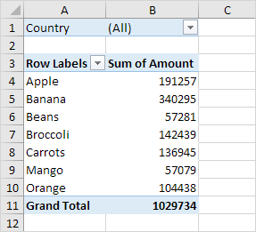
Change Pivot Table labels - Microsoft Community Answer Ashish Mathur Article Author Replied on April 21, 2015 Hi, You may rename the Pivot Table titles as XXXXX i.e. space after the XXXXX. Regards, Ashish Mathur Report abuse 1 person found this reply helpful · Was this reply helpful? Yes No Replies (1) How to make row labels on same line in pivot table? - ExtendOffice As we all know, the pivot table has several layout form, the tabular form may help us to put the row labels next to each other. Please do as follows: 1. Click any cell in your pivot table, and the PivotTable Tools tab will be displayed. 2. Under the PivotTable Tools tab, click Design > Report Layout > Show in Tabular Form, see screenshot: 3. Data Labels in Excel Pivot Chart (Detailed Analysis) Changing Appearance of Pivot Chart Labels We can change how the data label looks in order to have more clarity in the Pivot Chart. Steps Next, we will try to change the way the Data Labels look. We need to create the Pivot Table and the Chart the same way before. Then we click on the Plus sign top right corner of the Chart. Change language of auto-generated labels in pivot tables In pivot tables, some auto-generated labels in the field totals and filters use Russian words. For example, in the total row Итог Available Nights stands for Total Available Nights, and in the filter, (Все) stands for all items. I've sent the file to my client who uses English version, and he's seeing the same Russian words.
How to make row labels on same line in pivot table?
Sorting to your Pivot table row labels in custom order [quick tip] Create a pivot table with data set including sort order column. Add sort order column along with classification to the pivot table row labels area. Add the usual stuff to values area. Set up pivot table in tabular layout. Remove sub totals; Finally hide the column containing sort order. Your new pivot report is ready.
Pivot Table Filter in Excel | How to Filter Data in a Pivot ...
› xlpivot05Fix Excel Pivot Table Missing Data Field Settings Aug 31, 2022 · In the Pivot Table Field List, you can check a field name to add it to the pivot table layout. You have to do these one at a time though -- there isn't a "Select All" checkbox. With the following code, you can add all the unchecked fields to either the Row Labels area or to the Values area of the layout.
Excel- Automatically change the Pivot Table source data range ...
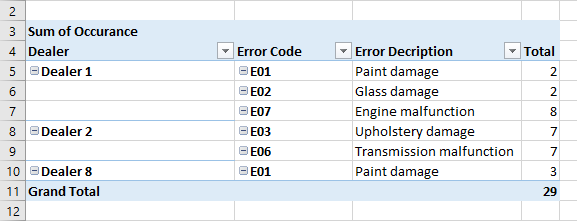
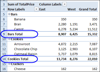
Change Excel Pivot Table Subtotal Text The text that you enter will apply to all the subtotals in that field. Type a New Subtotal Label When you type a new subtotal label, you can include the item name, or omit it. For example, if you select the Bars Total label in cell A9, and type "Subtotal", all of the items will change to that label. There is no item name in any subtotal label.
Manually Sorting Pivot Table Columns - Microsoft Community Hub
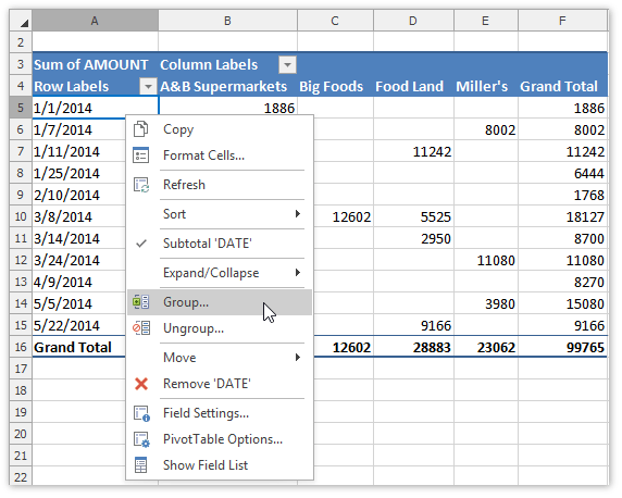
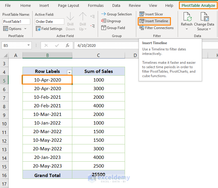
How to Change Date Format in Pivot Table in Excel - ExcelDemy To execute the task, follow the sequential steps. Firstly, click on the Group Selection option in the PivotTable Analyze tab while keeping the cursor over a cell of the Order Date (Row Labels). Secondly, you'll get the following dialog box namely Grouping. And choose Years from the options.
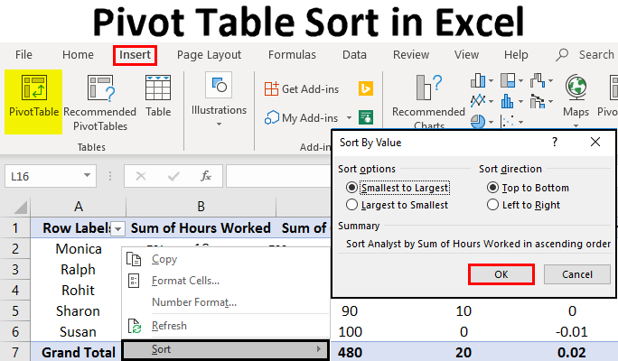
Pivot Table Sort in Excel | How to Sort Pivot Table Columns ...
Design the layout and format of a PivotTable Change a PivotTable to compact, outline, or tabular form Change the way item labels are displayed in a layout form Change the field arrangement in a PivotTable Add fields to a PivotTable Copy fields in a PivotTable Rearrange fields in a PivotTable Remove fields from a PivotTable Change the layout of columns, rows, and subtotals

How to Move Excel Pivot Table Labels Quick Tricks
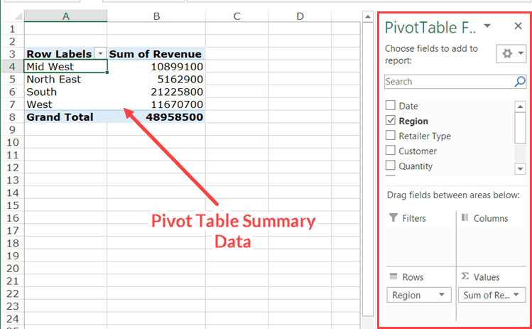
Pivot Table Tips | Exceljet On the Insert tab of the ribbon, click the PivotTable button. In the Create PivotTable dialog box, check the data and click OK. Drag a "label" field into the Row Labels area (e.g. customer) Drag a numeric field into the Values area (e.g. sales) A basic pivot table in about 30 seconds.
Pivot Table: Percentage of Total Calculations in Excel ...
How to rename group or row labels in Excel PivotTable? - ExtendOffice Click at the PivotTable, then click Analyze tab and go to the Active Field textbox. 2. Now in the Active Field textbox, the active field name is displayed, you can change it in the textbox. You can change other Row Labels name by clicking the relative fields in the PivotTable, then rename it in the Active Field textbox.
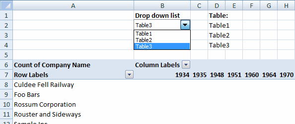
Change PivotTable data source using a drop-down list
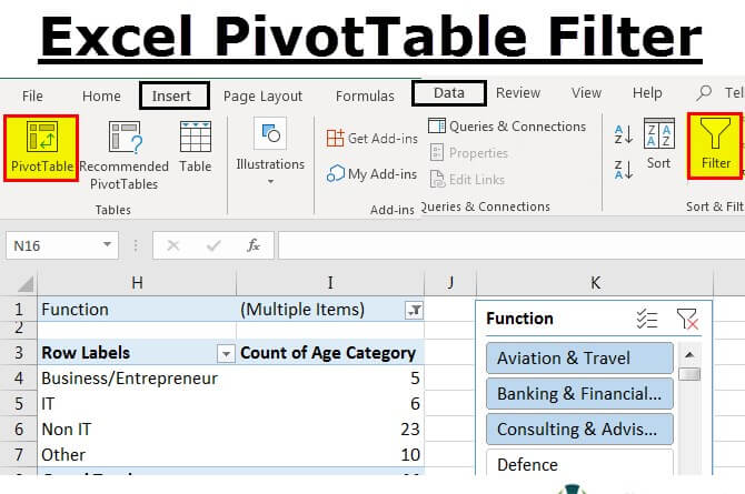
How to Use Excel Pivot Table Label Filters - Contextures Excel Tips To change the Pivot Table option, and allow multiple filters, follow these steps: Right-click a cell in the pivot table, and click PivotTable Options. In the PivotTable Options dialog box, click the Totals & Filters tab. In the Filters section, add a check mark to 'Allow multiple filters per field.'. Click the OK button, to apply the setting ...
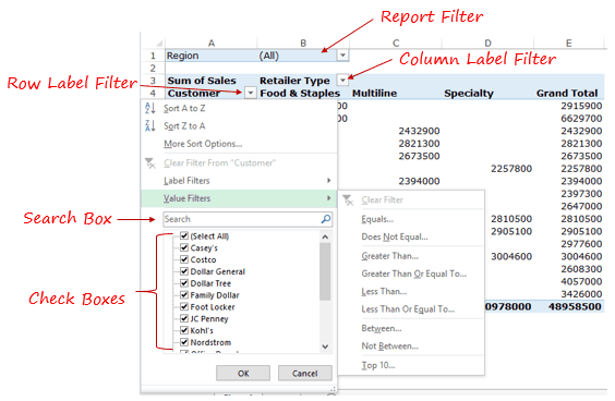
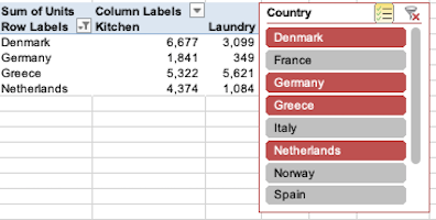
How to Filter Data in a Pivot Table in Excel
Pivot Table column label from horizontal to vertical Pivot Table column label from horizontal to vertical. After pivot table and with grouping, some column labels have been showed but the caption is on the top. What i want is put the column header at the left of the row as vertical red text show as below. However, i cannot do this, it said "We cant change this part of pivot table".

Remove Sum of in Pivot Table Headings – Contextures Blog
Automatic Row And Column Pivot Table Labels - How To Excel At Excel Select the Insert Tab Hit Pivot Table icon Next select Pivot Table option Select a table or range option Select to put your Table on a New Worksheet or on the current one, for this tutorial select the first option Click Ok The Options and Design Tab will appear under the Pivot Table Tool
How to Create a Pivot Table in Excel: A Step-by-Step Tutorial
Edit PivotTable Values - Excel University Step 1: Select a corresponding label cell. The first step for adding a Calculated Item is to tell Excel which field the new item belongs to. The way we communicate this to Excel is by selecting a corresponding report label cell. Let's unpack this for a second. A Calculated Item is a PivotTable formula that operates on items within a field.

Pivot table row labels side by side – Excel Tutorial
Pivot Table "Row Labels" Header Frustration - Microsoft Community Hub Pivot Table "Row Labels" Header Frustration. Discussion Options. Janie1964. Occasional Visitor. Jul 28 2021 12:03 PM.
Group Items in a Pivot Table | DevExpress End-User Documentation
› excel-pivot-taHow to Create Excel Pivot Table (Includes practice file) Jun 28, 2022 · The area to the left results from your selections from [1] and [2]. You’ll see that the only difference I made in the last pivot table was to drag the AGE GROUP field underneath the PRECINCT field in the Row Labels quadrant. How to Create Excel Pivot Table. There are several ways to build a pivot table.

EXCEL: SETTING PIVOT TABLE DEFAULTS - Strategic Finance
Change Pivot Table Data Headings and Blanks Change (Blank) Labels Another formatting fix that you can make is to get rid of the labels that say " (Blank")". These appear if cells are blank in the source data, and you add those fields to the row or column labels area. Excel shows an error message if you just try to delete those labels, but you can use a space character to replace them.
Rename Excel PivotTable headings - Office Watch
How to Move Pivot Table Labels - Contextures Excel Tips Right-click on the label that you want to move Click the Move command Click one of the Move subcommands, such as Move [item name] Up The existing labels shift down, and the moved label takes its new position. Type Over Another Label To move a pivot table label to a different position in the list, you can type its name over another label.
MS Excel 2016: How to Change the Name of a Pivot Table
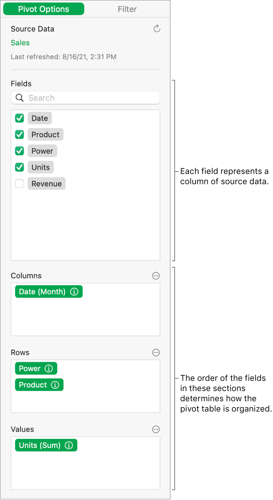
Create and edit pivot tables - Google Workspace Learning Center Edit a pivot table. Next to the pivot table, click Edit to open the pivot table editor. Add data —Depending on where you want to add data, under Rows, Columns, or Values, click Add. Change row or column names —Double-click a Row or Column name and enter a new name. Change sort order or column —Under Rows or Columns, click the Down arrow ...
How to rename group or row labels in Excel PivotTable?
› excel-pivot-table-formatHow to Format Excel Pivot Table - Contextures Excel Tips Jun 22, 2022 · Video: Change Pivot Table Labels. Watch this short video tutorial to see how to make these changes to the pivot table headings and labels. Get the Sample File. No Macros: To experiment with pivot table styles and formatting, download the sample file. The zipped file is in xlsx format, and and does NOT contain any macros.
Centre Column Headings in Excel Pivot Table | Excel Pivot Tables
› excel-pivot-table-subtotalsExcel Pivot Table Subtotals Examples Videos Workbooks Oct 10, 2022 · In the pivot table below, the Technician Count field was added below District, and the District field now has a subtotal after each District name. Hide All Subtotals. In a new pivot table, when you add multiple fields to the Row Labels or column Labels areas, subtotals are automatically shown for the outer fields.
Group Pivot Table Items in Excel (Easy Tutorial)
Change row label in Pivot Table with VBA | MrExcel Message Board If they appear as columns they are not row labels. If you want to change a field name between the source table and the pivot table I suggest you do this in SQL. So if the source data has fields Type and Manufacturer but you want them to be Type and Country in the pivot table it'd be like this, SELECT Type, Manufacturer AS [Country]
Change how pivot table data is sorted, grouped, and more in ...
Pivot Table shows row labels instead of field name - YouTube 00:00 Pivot table not showing column names, says 'Row Labels'00:13 Remove 'Row Labels', leave blank00:20 Show the column names in the Pivot TableChange your ...

Automatic Row And Column Pivot Table Labels
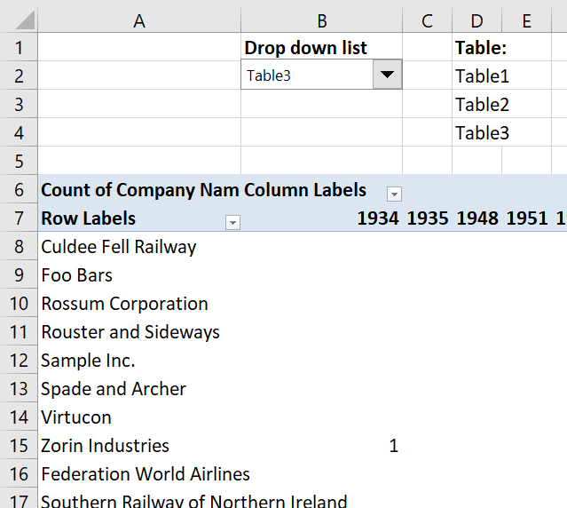
Change PivotTable data source using a drop-down list
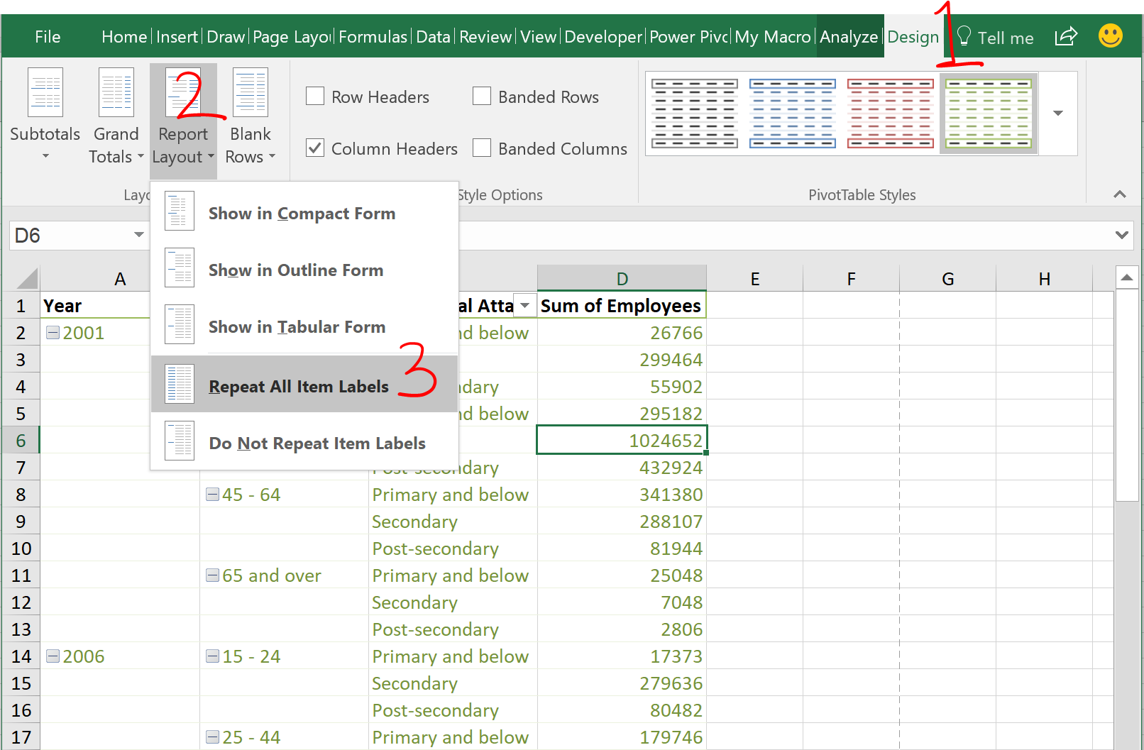
Repeat all item labels in Pivot Table (aka Fill in the blanks ...
How to rename group or row labels in Excel PivotTable?
How to Change the Pivot Table Layout in Your Excel Reports ...
How to Change Date Format in Pivot Table in Excel - ExcelDemy

Pivot table row labels in separate columns • AuditExcel.co.za

How to Use Excel Pivot Table Label Filters
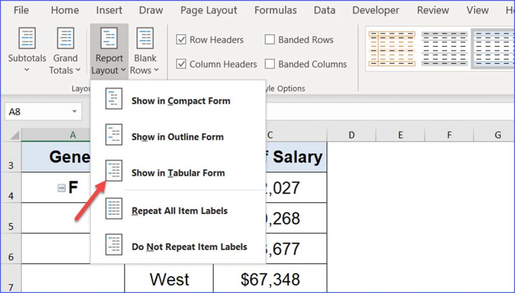
How to Change Pivot Table in Tabular Form - ExcelNotes
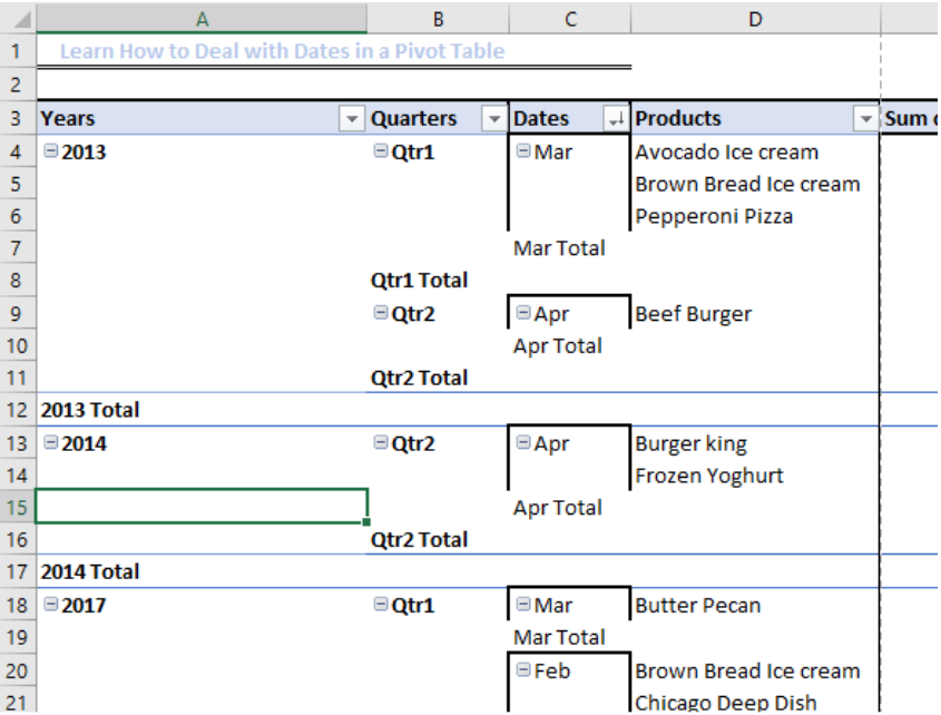
Learn How to Deal with Dates in a Pivot Table | Excelchat

Pivot table: How to show percentage change between quarter 1 ...
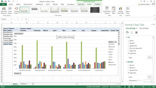
How to Customize Your Excel Pivot Chart and Axis Titles - dummies
How to Delete a Pivot Table in Excel (Easy Step-by-Step Guide)
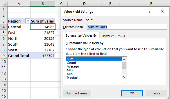
How to Use Pivot Table Field Settings and Value Field Setting
Pivot table row labels side by side – Excel Tutorial
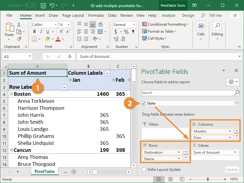
Add Multiple Columns to a Pivot Table | CustomGuide

Excel Pivot Tables: Insert Calculated Fields & Calculated ...
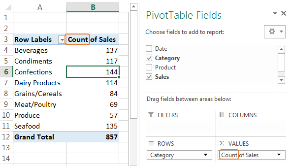
Excel PivotTable Default to SUM instead of COUNT
How to make row labels on same line in pivot table?

Remove Group Heading Excel Pivot Table - Stack Overflow
Automatic Default Number Formatting in Excel Pivot Tables ...
How to Change Pivot Table Name
Change Excel Pivot Table Subtotal Text | Excel Pivot Tables
Post a Comment for "43 change pivot table labels"