40 change data labels in excel chart
Move data labels - support.microsoft.com Click any data label once to select all of them, or double-click a specific data label you want to move. Right-click the selection > Chart Elements > Data Labels arrow, and select the placement option you want. Different options are available for different chart types. Edit titles or data labels in a chart - support.microsoft.com Change the position of data labels. You can change the position of a single data label by dragging it. You can also place data labels in a standard position relative to their data markers. Depending on the chart type, you can choose from a variety of positioning options. On a chart, do one of the following:
How to Make a Pie Chart in Excel & Add Rich Data Labels to The Chart! Sep 08, 2022 · A pie chart is used to showcase parts of a whole or the proportions of a whole. There should be about five pieces in a pie chart if there are too many slices, then it’s best to use another type of chart or a pie of pie chart in order to showcase the data better. In this article, we are going to see a detailed description of how to make a pie chart in excel.
Change data labels in excel chart
What Are Data Labels in Excel (Uses & Modifications) - ExcelDemy Removing Data Labels from an Excel Chart: To erase data labels from an Excel chart, please follow the steps below. Steps: Simply click on the chart that you would like to remove the data labels from. It shows the Chart Tools, including the Design and also Format tabs. How to make a bar graph in Excel - Ablebits.com Like other Excel chart types, bar graphs allow for many customizations with regard to the chart title, axes, data labels, and so on. The following resources explain the detailed steps: Adding the chart title; Customizing chart axes; Adding data labels; Adding, moving and formatting the chart legend; Showing or hiding the gridlines; Editing data ... Add a Horizontal Line to an Excel Chart - Peltier Tech Sep 11, 2018 · This tutorial shows how to add horizontal lines to several common types of Excel chart. We won’t even talk about trying to draw lines using the items on the Shapes menu. Since they are drawn freehand (or free-mouse), they aren’t positioned accurately. Since they are independent of the chart’s data, they may not move when the data changes.
Change data labels in excel chart. Once the connection is made, I am calling a function named createChart ... Use a named control instead of "WebBrowser1". hi, i am trying to create a combined chart - line and column. i am using chart column widget and i am using the advanced format highchart json to add another series (see the photo attached). the first series i just enter the label and the value in the column widget but i cant seem to figure out ... Change the format of data labels in a chart To get there, after adding your data labels, select the data label to format, and then click Chart Elements > Data Labels > More Options. To go to the appropriate area, click one of the four icons ( Fill & Line, Effects, Size & Properties ( Layout & Properties in Outlook or Word), or Label Options) shown here. Change the format of data labels in a chart To get there, after adding your data labels, select the data label to format, and then click Chart Elements > Data Labels > More Options. To go to the appropriate area, click one of the four icons ( Fill & Line, Effects, Size & Properties ( Layout & Properties in Outlook or Word), or Label Options) shown here. How to Rename a Data Series in Microsoft Excel - How-To Geek To do this, right-click your graph or chart and click the "Select Data" option. This will open the "Select Data Source" options window. Your multiple data series will be listed under the "Legend Entries (Series)" column. To begin renaming your data series, select one from the list and then click the "Edit" button.
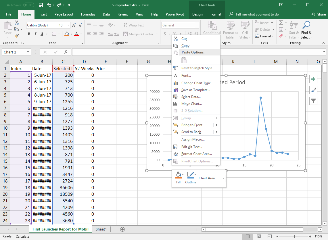
How to add data labels from different column in an Excel chart? Right click the data series in the chart, and select Add Data Labels > Add Data Labels from the context menu to add data labels. 2. Click any data label to select all data labels, and then click the specified data label to select it only in the chart. 3. Change the format of data labels in a chart To get there, after adding your data labels, select the data label to format, and then click Chart Elements > Data Labels > More Options. To go to the appropriate area, click one of the four icons ( Fill & Line, Effects, Size & Properties ( Layout & Properties in Outlook or Word), or Label Options) shown here. Data Labels in Excel Pivot Chart (Detailed Analysis) Next open Format Data Labels by pressing the More options in the Data Labels. Then on the side panel, click on the Value From Cells. Next, in the dialog box, Select D5:D11, and click OK. Right after clicking OK, you will notice that there are percentage signs showing on top of the columns. 4. Changing Appearance of Pivot Chart Labels How to create Custom Data Labels in Excel Charts - Efficiency 365 Create the chart as usual. Add default data labels. Click on each unwanted label (using slow double click) and delete it. Select each item where you want the custom label one at a time. Press F2 to move focus to the Formula editing box. Type the equal to sign. Now click on the cell which contains the appropriate label.
How to I rotate data labels on a column chart so that they are ... To change the text direction, first of all, please double click on the data label and make sure the data are selected (with a box surrounded like following image). Then on your right panel, the Format Data Labels panel should be opened. Go to Text Options > Text Box > Text direction > Rotate Modify Excel Chart Data Range | CustomGuide The new data needs to be in cells adjacent to the existing chart data. Rename a Data Series. Charts are not completely tied to the source data. You can change the name and values of a data series without changing the data in the worksheet. Select the chart; Click the Design tab. Click the Select Data button. Edit titles or data labels in a chart - support.microsoft.com The first click selects the data labels for the whole data series, and the second click selects the individual data label. Right-click the data label, and then click Format Data Label or Format Data Labels. Click Label Options if it's not selected, and then select the Reset Label Text check box. Top of Page How to Edit Pie Chart in Excel (All Possible Modifications) How to Edit Pie Chart in Excel 1. Change Chart Color 2. Change Background Color 3. Change Font of Pie Chart 4. Change Chart Border 5. Resize Pie Chart 6. Change Chart Title Position 7. Change Data Labels Position 8. Show Percentage on Data Labels 9. Change Pie Chart's Legend Position 10. Edit Pie Chart Using Switch Row/Column Button 11.
Move data labels
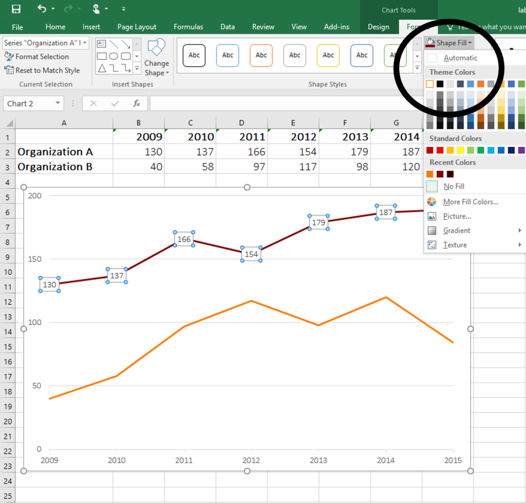
How to Change Excel Chart Data Labels to Custom Values? - Chandoo.org May 05, 2010 · Now, click on any data label. This will select “all” data labels. Now click once again. At this point excel will select only one data label. Go to Formula bar, press = and point to the cell where the data label for that chart data point is defined. Repeat the process for all other data labels, one after another. See the screencast.

Color Negative Chart Data Labels in Red with downward arrow
How to Add Total Data Labels to the Excel Stacked Bar Chart Apr 03, 2013 · Step 4: Right click your new line chart and select “Add Data Labels” Step 5: Right click your new data labels and format them so that their label position is “Above”; also make the labels bold and increase the font size. Step 6: Right click the line, select “Format Data Series”; in the Line Color menu, select “No line”

Add data labels and callouts to charts in Excel 365 ...
Change axis labels in a chart - support.microsoft.com Right-click the category labels you want to change, and click Select Data. In the Horizontal (Category) Axis Labels box, click Edit. In the Axis label range box, enter the labels you want to use, separated by commas. For example, type Quarter 1,Quarter 2,Quarter 3,Quarter 4. Change the format of text and numbers in labels
Change Horizontal Axis Values in Excel 2016 - AbsentData
How to change Axis labels in Excel Chart - A Complete Guide Right-click the horizontal axis (X) in the chart you want to change. In the context menu that appears, click on Select Data…. A Select Data Source dialog opens. In the area under the Horizontal (Category) Axis Labels box, click the Edit command button. Enter the labels you want to use in the Axis label range box, separated by commas.

how to add data labels into Excel graphs — storytelling with data
How to Create a Dynamic Chart Range in Excel - Trump Excel The above steps would insert a line chart which would automatically update when you add more data to the Excel table. Note that while adding new data automatically updates the chart, deleting data would not completely remove the data points. For example, if you remove 2 data points, the chart will show some empty space on the right.

How-to Use Data Labels from a Range in an Excel Chart - Excel ...
Chart Axis - Use Text Instead of Numbers - Automate Excel Change Labels. While clicking the new series, select the + Sign in the top right of the graph; Select Data Labels; Click on Arrow and click Left . 4. Double click on each Y Axis line type = in the formula bar and select the cell to reference . 5. Click on the Series and Change the Fill and outline to No Fill . 6.

Solved: How to show all detailed data labels of pie chart ...
How to Change Excel Chart Data Labels to Custom Values? - Chandoo.org You can change data labels and point them to different cells using this little trick. First add data labels to the chart (Layout Ribbon > Data Labels) Define the new data label values in a bunch of cells, like this: Now, click on any data label. This will select "all" data labels. Now click once again.

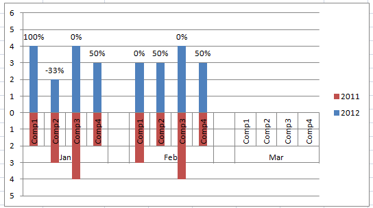
Excel: Clustered Column Chart with Percent of Month ...
Change the format of data labels in a chart To get there, after adding your data labels, select the data label to format, and then click Chart Elements > Data Labels > More Options. To go to the appropriate area, click one of the four icons ( Fill & Line , Effects , Size & Properties ( Layout & Properties in Outlook or Word), or Label Options ) shown here.

Change the format of data labels in a chart
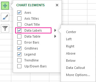
Add or remove data labels in a chart - support.microsoft.com Click the data series or chart. To label one data point, after clicking the series, click that data point. In the upper right corner, next to the chart, click Add Chart Element > Data Labels. To change the location, click the arrow, and choose an option. If you want to show your data label inside a text bubble shape, click Data Callout.
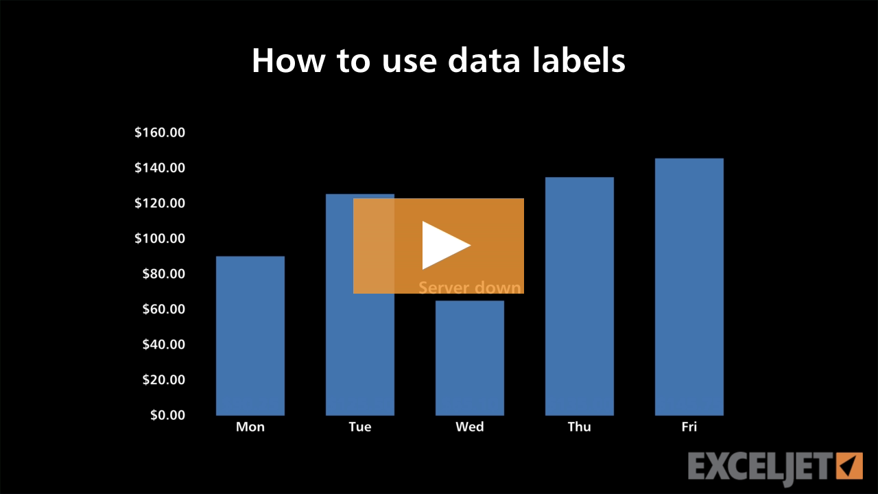
Excel tutorial: How to use data labels
How to add or move data labels in Excel chart? - ExtendOffice In Excel 2013 or 2016. 1. Click the chart to show the Chart Elements button . 2. Then click the Chart Elements, and check Data Labels, then you can click the arrow to choose an option about the data labels in the sub menu. See screenshot: In Excel 2010 or 2007. 1. click on the chart to show the Layout tab in the Chart Tools group. See ...

Excel Charts - Aesthetic Data Labels
How to Change Axis Labels in Excel (3 Easy Methods) Firstly, right-click the category label and click Select Data > Click Edit from the Horizontal (Category) Axis Labels icon. Then, assign a new Axis label range and click OK. Now, press OK on the dialogue box. Finally, you will get your axis label changed. That is how we can change vertical and horizontal axis labels by changing the source.

Change the format of data labels in a chart
Is there a way to change the order of Data Labels? Answer Rena Yu MSFT Microsoft Agent | Moderator Replied on April 4, 2018 Hi Keith, I got your meaning. Please try to double click the the part of the label value, and choose the one you want to show to change the order. Thanks, Rena ----------------------- * Beware of scammers posting fake support numbers here.

Custom data labels in a chart
How to change chart axis labels' font color and size in Excel? We can easily change all labels' font color and font size in X axis or Y axis in a chart. Just click to select the axis you will change all labels' font color and size in the chart, and then type a font size into the Font Size box, click the Font color button and specify a font color from the drop down list in the Font group on the Home tab. See below screen shot:

Change Horizontal Axis Values in Excel 2016 - AbsentData
Excel Charts - Aesthetic Data Labels - tutorialspoint.com Data Label Positions. To place the data labels in the chart, follow the steps given below. Step 1 − Click the chart and then click chart elements. Step 2 − Select Data Labels. Click to see the options available for placing the data labels. Step 3 − Click Center to place the data labels at the center of the bubbles.

Custom Excel Chart Label Positions • My Online Training Hub
Add a Horizontal Line to an Excel Chart - Peltier Tech Sep 11, 2018 · This tutorial shows how to add horizontal lines to several common types of Excel chart. We won’t even talk about trying to draw lines using the items on the Shapes menu. Since they are drawn freehand (or free-mouse), they aren’t positioned accurately. Since they are independent of the chart’s data, they may not move when the data changes.

How to add or move data labels in Excel chart?
How to make a bar graph in Excel - Ablebits.com Like other Excel chart types, bar graphs allow for many customizations with regard to the chart title, axes, data labels, and so on. The following resources explain the detailed steps: Adding the chart title; Customizing chart axes; Adding data labels; Adding, moving and formatting the chart legend; Showing or hiding the gridlines; Editing data ...

Change Chart Data Labels : Chart Data « Chart « Microsoft ...
What Are Data Labels in Excel (Uses & Modifications) - ExcelDemy Removing Data Labels from an Excel Chart: To erase data labels from an Excel chart, please follow the steps below. Steps: Simply click on the chart that you would like to remove the data labels from. It shows the Chart Tools, including the Design and also Format tabs.
How to Place Labels Directly Through Your Line Graph in ...

Change the format of data labels in a chart

Add or remove data labels in a chart

Directly Labeling Excel Charts - PolicyViz

Change color of data label placed, using the 'best fit ...

How to Place Labels Directly Through Your Line Graph in ...
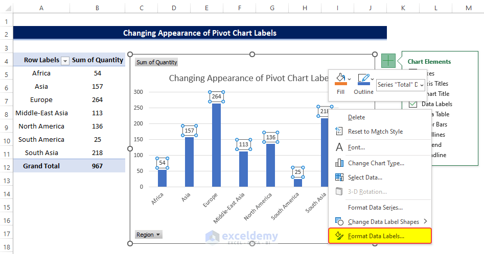
Data Labels in Excel Pivot Chart (Detailed Analysis) - ExcelDemy

Adding rich data labels to charts in Excel 2013 | Microsoft ...
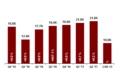
Add % Difference Data Labels to Excel Horizontal Tornado ...

How to add data labels from different column in an Excel chart?

How to Make Pie Chart with Labels both Inside and Outside ...

excel - VBA Change Data Labels on a Stacked Column chart from ...

Custom Data Labels with Colors and Symbols in Excel Charts ...

How to Add Total Data Labels to the Excel Stacked Bar Chart ...

Adding rich data labels to charts in Excel 2013 | Microsoft ...
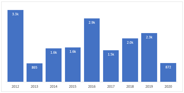
Format Chart Numbers as Thousands or Millions — Excel ...

Excel charts: add title, customize chart axis, legend and ...

Change the format of data labels in a chart
Excel Clustered Column chart data labels positioning ...

How to Add Two Data Labels in Excel Chart (with Easy Steps ...

Is it possible to conditionally format Data Labels on a ...

Apply Custom Data Labels to Charted Points - Peltier Tech

How to hide zero data labels in chart in Excel?
Post a Comment for "40 change data labels in excel chart"