44 chart data labels excel

Change the format of data labels in a chart To get there, after adding your data labels, select the data label to format, and then click Chart Elements > Data Labels > More Options. To go to the appropriate area, click one of the four icons ( Fill & Line, Effects, Size & Properties ( Layout & Properties in Outlook or Word), or Label Options) shown here. How to Change Excel Chart Data Labels to Custom Values? First add data labels to the chart (Layout Ribbon > Data Labels) Define the new data label values in a bunch of cells, like this: Now, click on any data label. This will select "all" data labels. Now click once again. At this point excel will select only one data label.

Add / Move Data Labels in Charts - Excel & Google Sheets We'll start with the same dataset that we went over in Excel to review how to add and move data labels to charts. Add and Move Data Labels in Google Sheets Double Click Chart Select Customize under Chart Editor Select Series 4. Check Data Labels 5. Select which Position to move the data labels in comparison to the bars.

Chart data labels excel

Add a DATA LABEL to ONE POINT on a chart in Excel Steps shown in the video above: Click on the chart line to add the data point to. All the data points will be highlighted. Click again on the single point that you want to add a data label to. Right-click and select ' Add data label ' This is the key step! Right-click again on the data point itself (not the label) and select ' Format data label '. Add data labels and callouts to charts in Excel 365 | EasyTweaks.com The steps that I will share in this guide apply to Excel 2021 / 2019 / 2016. Step #1: After generating the chart in Excel, right-click anywhere within the chart and select Add labels . Note that you can also select the very handy option of Adding data Callouts. How to Add Data Labels in Excel - Excelchat | Excelchat After inserting a chart in Excel 2010 and earlier versions we need to do the followings to add data labels to the chart; Click inside the chart area to display the Chart Tools. Figure 2. Chart Tools Click on Layout tab of the Chart Tools. In Labels group, click on Data Labels and select the position to add labels to the chart. Figure 3.

Chart data labels excel. Excel tutorial: How to use data labels Generally, the easiest way to show data labels to use the chart elements menu. When you check the box, you'll see data labels appear in the chart. If you have more than one data series, you can select a series first, then turn on data labels for that series only. You can even select a single bar, and show just one data label. How to add or move data labels in Excel chart? - ExtendOffice In Excel 2013 or 2016. 1. Click the chart to show the Chart Elements button . 2. Then click the Chart Elements, and check Data Labels, then you can click the arrow to choose an option about the data labels in the sub menu. See screenshot: In Excel 2010 or 2007. 1. click on the chart to show the Layout tab in the Chart Tools group. See ... How to add data labels from different column in an Excel chart? Right click the data series in the chart, and select Add Data Labels > Add Data Labels from the context menu to add data labels. 2. Click any data label to select all data labels, and then click the specified data label to select it only in the chart. 3. How to create a chart with both percentage and value in Excel? In the Format Data Labels pane, please check Category Name option, and uncheck Value option from the Label Options, and then, you will get all percentages and values are displayed in the chart, see screenshot: 15.

How to Create a Bar Chart With Labels Inside Bars in Excel In the chart, right-click the Series "# Footballers" Data Labels and then, on the short-cut menu, click Format Data Labels. 8. In the Format Data Labels pane, under Label Options selected, set the Label Position to Inside End. 9. Next, in the chart, select the Series 2 Data Labels and then set the Label Position to Inside Base. 10. How to add axis label to chart in Excel? - ExtendOffice Click to select the chart that you want to insert axis label. 2. Then click the Charts Elements button located the upper-right corner of the chart. In the expanded menu, check Axis Titles option, see screenshot: 3. And both the horizontal and vertical axis text boxes have been added to the chart, then click each of the axis text boxes and enter ... Adding rich data labels to charts in Excel 2013 | Microsoft 365 Blog Putting a data label into a shape can add another type of visual emphasis. To add a data label in a shape, select the data point of interest, then right-click it to pull up the context menu. Click Add Data Label, then click Add Data Callout . The result is that your data label will appear in a graphical callout. How to Use Cell Values for Excel Chart Labels Select the chart, choose the "Chart Elements" option, click the "Data Labels" arrow, and then "More Options." Uncheck the "Value" box and check the "Value From Cells" box. Select cells C2:C6 to use for the data label range and then click the "OK" button. The values from these cells are now used for the chart data labels.

Custom data labels in a chart - Get Digital Help Jan 21, 2020 — Press with right mouse button on on any data series displayed in the chart. · Press with mouse on "Add Data Labels". · Press with mouse on Add ... Chart.ApplyDataLabels method (Excel) | Microsoft Docs ApplyDataLabels ( Type, LegendKey, AutoText, HasLeaderLines, ShowSeriesName, ShowCategoryName, ShowValue, ShowPercentage, ShowBubbleSize, Separator) expression A variable that represents a Chart object. Parameters Example This example applies category labels to series one on Chart1. VB Copy Charts ("Chart1").SeriesCollection (1). How To Use Dynamic Data Labels To Create Interactive Excel Charts To create a column chart with dynamic data labels, you need to follow these given steps. Select the data & Create a Combo Chart. Now select the column chart for revenue data and a line chart with marker for data labels. Add Data Labels to the Line Chart With Marker. After then remove the Line Color and Marker Color. Custom Chart Data Labels In Excel With Formulas Follow the steps below to create the custom data labels. Select the chart label you want to change. In the formula-bar hit = (equals), select the cell reference containing your chart label's data. In this case, the first label is in cell E2. Finally, repeat for all your chart laebls.

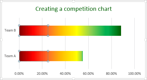
Creating a funny competition chart

Data Labels on Chart Series - Excelguru Applying data labels when the legend is selected will apply data labels to all the series in the chart. Your screen shot of data labels would suggest that the information is in fact the values of the first series rather than multiple #N/As. Select the actual series before applying data labels.

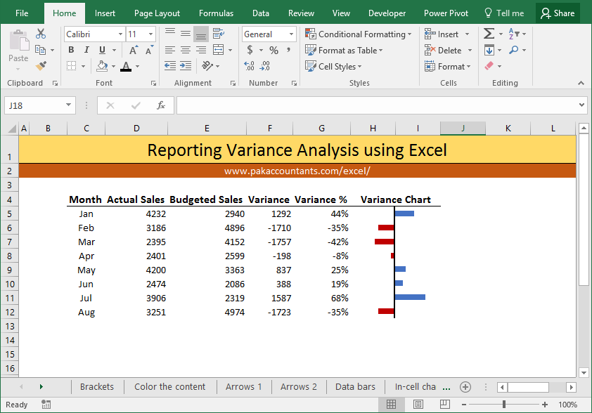
10 ways to present variance analysis reports in Excel - PakAccountants.com

Edit titles or data labels in a chart - support.microsoft.com On a chart, click one time or two times on the data label that you want to link to a corresponding worksheet cell. The first click selects the data labels for the whole data series, and the second click selects the individual data label. Right-click the data label, and then click Format Data Label or Format Data Labels.

Excel Course: Inserting Graphs

How to create Custom Data Labels in Excel Charts Create the chart as usual. Add default data labels. Click on each unwanted label (using slow double click) and delete it. Select each item where you want the custom label one at a time. Press F2 to move focus to the Formula editing box. Type the equal to sign. Now click on the cell which contains the appropriate label.

Share :