41 how to add axis labels in excel bar graph

Doing the Math: Analysis of Forces in a Truss Bridge ... Bar forces do not produce any moments or rotation at the joint, then only two equations of statics are used to find the unknown forces: ∑F_x = 0, ∑F_y = 0 moment of a force: In Statics, it is a measure of the tendency of a force to cause a body to rotate about a specific point or axis. The magnitude of the moment is defined as the product ... Figures - APA 6th referencing style - Library Guides at ... Provide each figure with a brief but explanatory title. This should appear next to the figure number. A caption should be included the bottom of the figure to acknowledge that the figure has been reproduced from another source. Include the full reference in the reference list. An example can be found here.

superuser.com › questions › 1195816Excel Chart not showing SOME X-axis labels - Super User Apr 05, 2017 · On the sidebar, click on "CHART OPTIONS" and select "Horizontal (Category) Axis" from the drop down menu. Four icons will appear below the menu bar. The right most icon looks like a bar graph. Click that. A navigation bar with several twistys will appear below the icon ribbon. Click on the "LABELS" twisty.

How to add axis labels in excel bar graph

how to add a line in google sheets graph Uncheck the box next to Link to spreadsheet if you want the chart to stand alone. Step 4: Add a secondary Y axis. From the drop-down menu, click the Chart option. - Start entering the values for X-axis and give a column name. Click Add under . The chart will be created as shown in the picture below. Crosstabs - SPSS Tutorials - LibGuides at Kent State ... The dimensions of the crosstab refer to the number of rows and columns in the table. (The "total" row/column are not included.) The table dimensions are reported as as RxC, where R is the number of categories for the row variable, and C is the number of categories for the column variable.. Additionally, a "square" crosstab is one in which the row and column variables have the same number of ... Table of keyboard shortcuts - Wikipedia In computing, a keyboard shortcut is a sequence or combination of keystrokes on a computer keyboard which invokes commands in software.. Most keyboard shortcuts require the user to press a single key or a sequence of keys one after the other. Other keyboard shortcuts require pressing and holding several keys simultaneously (indicated in the tables below by the + sign).

How to add axis labels in excel bar graph. › documents › excelHow to add data labels from different column in an Excel chart? This method will introduce a solution to add all data labels from a different column in an Excel chart at the same time. Please do as follows: 1. Right click the data series in the chart, and select Add Data Labels > Add Data Labels from the context menu to add data labels. 2. Reporting 2.0 - Create Report - Cornerstone OnDemand Reporting 2.0 - Create Report. Reports are created by clicking the Create Report button on the Reporting homepage. This will open the Create Report page for Reporting 2.0. Note: Users who belong to the LXP_Admin and LXP_Manager groups can only create reports by using the System Templates. Click here to download the list of Reporting 2.0 field descriptions, updated May 2022. Understand charts: Underlying data and chart ... Use the presentation description XML string to specify data representation Methods and properties supported in Unified Interface Charts display data visually by mapping textual values on two axes: horizontal (x) and vertical (y). The x axis is called the category axis and the y axis is called the series axis. Scatter plot - Junk Charts The basic chart form is a column chart that is curled up into a ball. The column chart is given colors that map to continents. All countries are grouped into five continents. The column chart can only take a single data series, so the 2019 fertility rate is chosen. Beyond this basic setup, the designer embellishes the chart with a trove of ...

Basic Excel Tutorial Excel is a cell-based working platform, and therefore it is more convenient to place the first and the second name on each column. However, while working on this data, you may need to merge the first and the second name in one column. This may be possible using the following methods: Method 1: Using the …. Read more. How to Customize Histograms in MATLAB - Video - MATLAB Now that we're working with a bar graph, we can quickly apply useful customizations. First, we'll modify the y-axis ticks to display percentages, and adjust the count to match. And as with any good graph, we should add a title, and label the axes. To learn more about histograms and other customizations for MATLAB graphs, check out the links ... Focus mode and full screen mode - how to zoom in to see ... To see a visual in full screen mode, first open it in focus mode and then select View > Full screen. Your selected content fills the entire screen. Once you're in full screen mode, navigate using either the menu bars at the top and bottom (reports) or the menu that appears when you move your cursor (dashboards and visuals). FNU | Moodle: Dashboard (GUEST) Greetings from the Office of the Registrar. The Office of the Registrar is conducting a survey on the FNU Complaints Portal and the FNU Text Free Platform. This survey is CONFIDENTIAL & ANONYMOUS. We invite you to participate in the survey as your feedback will assist us in the delivery of quality services by the Fiji National University.

Table and Matrix Visualization in Power BI | Power BI ... Step 1) To add a Matrix to your canvas, click on the Matrix option under Visualization Pane. Step 2) Now you can fill in the Matrix with data. In this demo, we drag and drop the Card Type in the Rows, Date in the column, and Amount in the values as shown below. It also shows the hierarchy for the date as Year, Quarter, Month, and Day. How To Add A Vertical Line To An Excel Chart (2022) Then open the Add Data Labels menu and click Add Data Labels. You should then see a data label appear next to your vertical line. Next, you'll likely want to reposition your data label to be directly over your vertical line. To do this, select and right-click on your data label. File: README — Documentation for axlsx (2.0.1) Generate 3D Pie, Line, Scatter and Bar Charts: With Axlsx chart generation and management is as easy as a few lines of code. You can build charts based off data in your worksheet or generate charts without any data in your sheet at all. Customize gridlines, label rotation and series colors as well. Microsoft Power BI Training | Beginner Course - Nexacu View our full Power BI Beginner course outline below. Microsoft Power BI Training - Beginner Course. 4.73. see reviews. Pre-Course: Power BI Beginner. 1:17. Learn to use Power BI to create interactive dashboards, custom reports, analyse data and share insights. $385.

Two-Level Axis Labels (Microsoft Excel)

how to add a line in google sheets graph We'll use mock width and height measurements for this example Step 2 Select the columns containing your data and open the Insert menu, then choose Chart Step 3 Choose the second data series dropdown, and set its axis . You can click Data range to change the data range that's included in your chart.

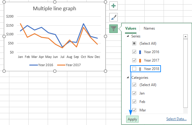
How To Make A Line Graph In Excel With Multiple Lines On Mac

Box Plots | JMP Background. Color Black White Red Green Blue Yellow Magenta Cyan Transparency Opaque Semi-Transparent Transparent. Window. Color Black White Red Green Blue Yellow Magenta Cyan Transparency Transparent Semi-Transparent Opaque. Font Size. 50% 75% 100% 125% 150% 175% 200% 300% 400%. Text Edge Style.

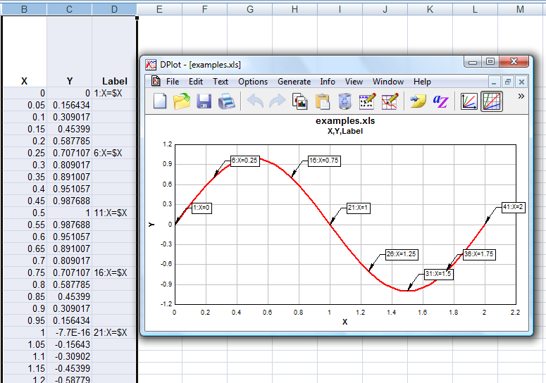
DPlot Windows software for Excel users to create presentation quality graphs

How to Format Excel Pivot Table - Contextures Excel Tips Follow these steps to copy a pivot table's values and formatting: Select the original pivot table, and copy it. Click the cell where you want to paste the copy. On the Excel Ribbon's Home tab, click the Dialog Launcher button in the Clipboard group . In the Clipboard, click on the pivot table copy, in the list of copied items..

r - Breaking value axis using ggplot2 - Stack Overflow

Chris Webb's BI Blog Chris Webb's BI Blog Power Query in Excel for the Mac. One of the priorities for the Excel Power Query team has been to get Power Query working in Excel on the Mac, and in the latest update we now have the Power Query Editor available. Data sources are still limited to files (CSV, Excel, XML, JSON), Excel tables/ranges, SharePoint, OData and SQL Server but they are ...

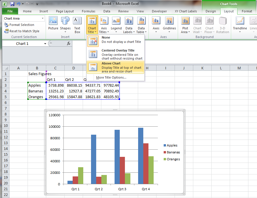
Link chart title to cell

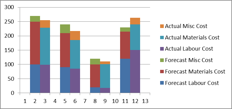
› excel › how-to-add-total-dataHow to Add Total Data Labels to the Excel Stacked Bar Chart Apr 03, 2013 · Step 4: Right click your new line chart and select “Add Data Labels” Step 5: Right click your new data labels and format them so that their label position is “Above”; also make the labels bold and increase the font size. Step 6: Right click the line, select “Format Data Series”; in the Line Color menu, select “No line”

Axis Labels That Don't Block Plotted Data - Peltier Tech Blog

Fixed- and Mixed-Effects Regression Models in R The graphs indicate that data points 52, 64, and 83 may be problematic. We will therefore statistically evaluate whether these data points need to be removed. In order to find out which data points require removal, we extract the influence measure statistics and add them to out data set.

Step-by-step tutorial on creating clustered stacked column bar charts (for free) | Excel Help HQ

Grouping Data - SPSS Tutorials - LibGuides at Kent State ... To split the data in a way that will facilitate group comparisons: Click Data > Split File. Select the option Compare groups. Double-click the variable Gender to move it to the Groups Based on field. When you are finished, click OK.

How to Make Your Excel Bar Chart Look Better – MBA Excel

› Make-a-Bar-Graph-in-ExcelHow to Make a Bar Graph in Excel: 9 Steps (with Pictures) May 02, 2022 · Add labels for the graph's X- and Y-axes. To do so, click the A1 cell (X-axis) and type in a label, then do the same for the B1 cell (Y-axis). For example, a graph measuring the temperature over a week's worth of days might have "Days" in A1 and "Temperature" in B1.

Share :